The maths explained series: Calculating the effect controls have on your risk profile

Cyber risk management

Friday, 30 May, 2025

Ray Morrison

Graph

Recap

In the first post in this series (Quantitative Risk Analysis), we looked at a methodology for calculating the risk profile of a single risk. This included plotting the changing likelihood of a risk event incurring a defined minimum loss.

In the second post (Compound risk calculations to show overall risk profiles), we looked at how to combine multiple risks together, and how these can be compared to show the impact of individual risks on the overall risk profile.

Fig. 1: Loss exceedance curve showing 2 individual risks and their combined risk

In this post, I will discuss how we can create a similar image to illustrate the impact that controls can have on your risk profile, and how to use this to identify those controls which best bring your risk profile within tolerance.

Calculating the impact of implementing controls

Let’s look at how we can calculate the effect that implementing different types of controls can have on our risk profile. As with all mathematical simulations it is possible to make this as simple or complicated as required, and we do this through the assumptions that we make when we create the model.

For this model, we will just look at single risk events, but the principles defined in (Compound risk calculations to show overall risk profiles) can equally be applied to the risk profiles we will create here, and vice versa.

Risk mitigation

Controls implemented to mitigate a risk can reduce either the impact of an event should it happen, the likelihood of the event occurring in the first place, or both. The effect of these controls is calculated before the simulation is run.

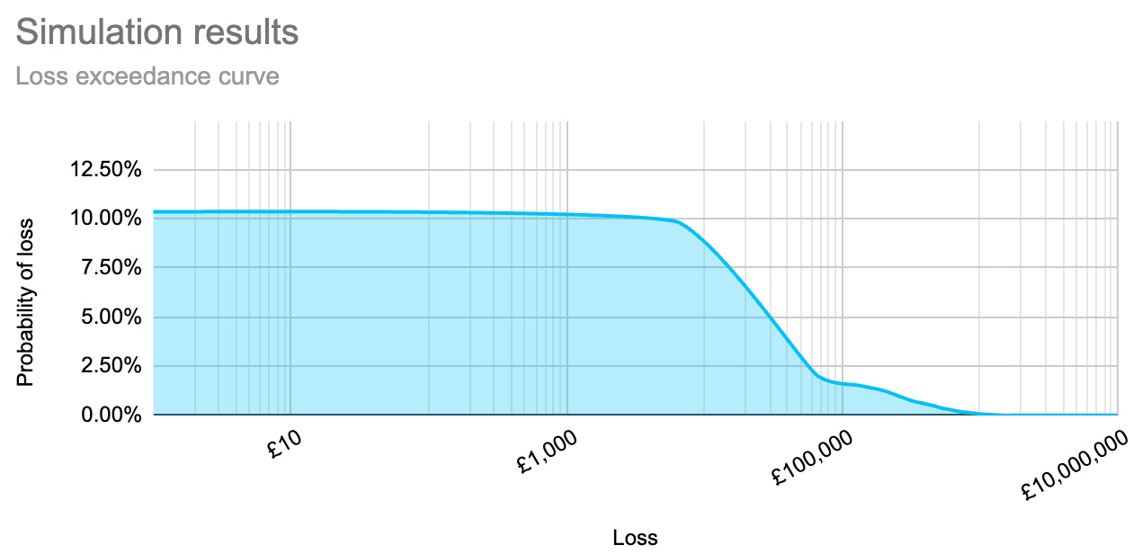
Let’s start with a risk which occurs once every 10 years:

Fig. 2: Binomial tree of a single risk

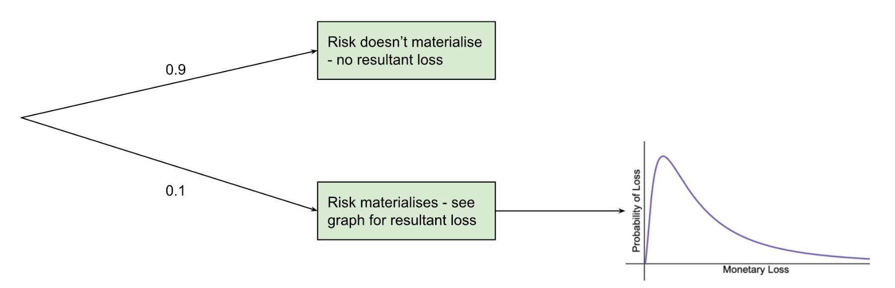
Which has a confidence interval of between £100k and £1M, so has the following risk profile:

Fig. 3: Loss exceedance curve showing the risk from fig. 2.

Reduce likelihood

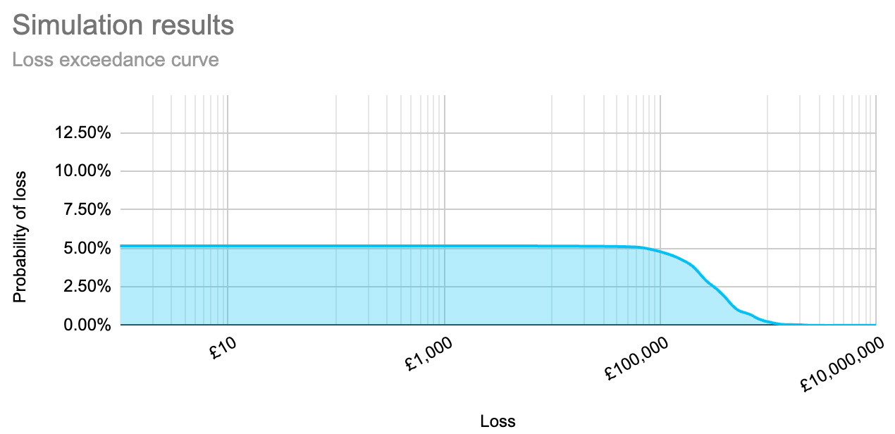
To reduce the impact of the risk, a control is implemented which industry intelligence shows reduces the likelihood of the event occurring from 10% to 5%.

This changes how often there is a loss.

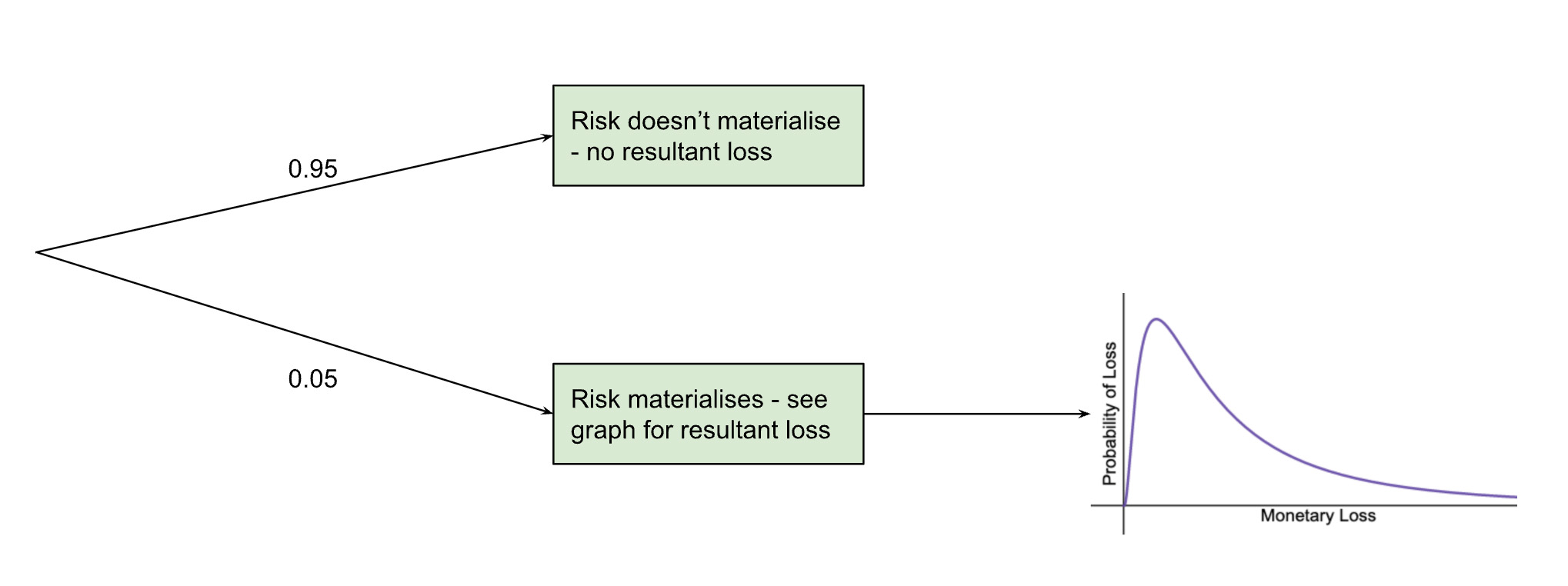
Fig. 4: Binomial tree of the risk from fig. 2, with a reduced likelihood.

And reduces the probability of a loss event. We can see this in the lower height of our risk profile. The control does not change the possible loss values: we can see the graph below extends to the right just as far as the untreated risk, and starts to go down at the same point.

Fig. 5: Loss exceedance curve showing the risk from fig. 4.

Reduce impact

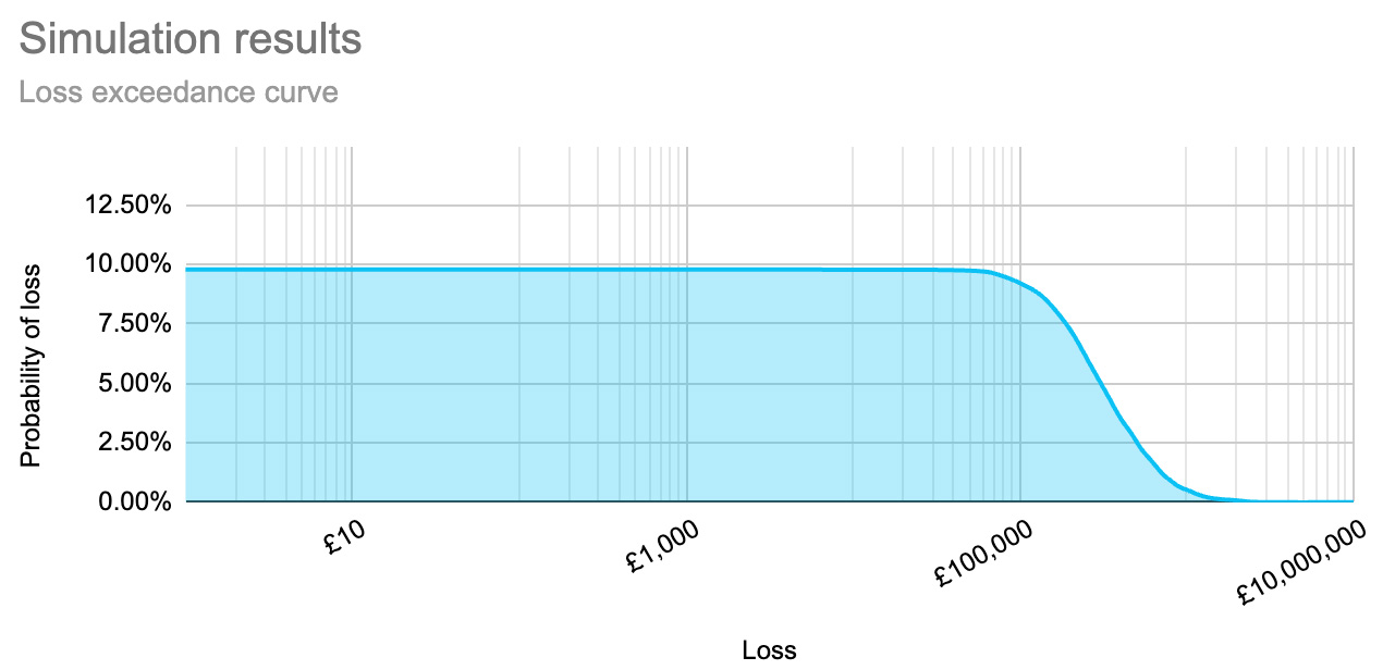
Alternatively, the organisation considers implementing a control which will reduce the impact of an event should it occur. In this case the probability of the event occurring is not reduced:

Fig. 6: Binomial tree of the risk from fig. 2, with a reduced impact.

But the confidence interval has been reduced to between £10k and £100k.

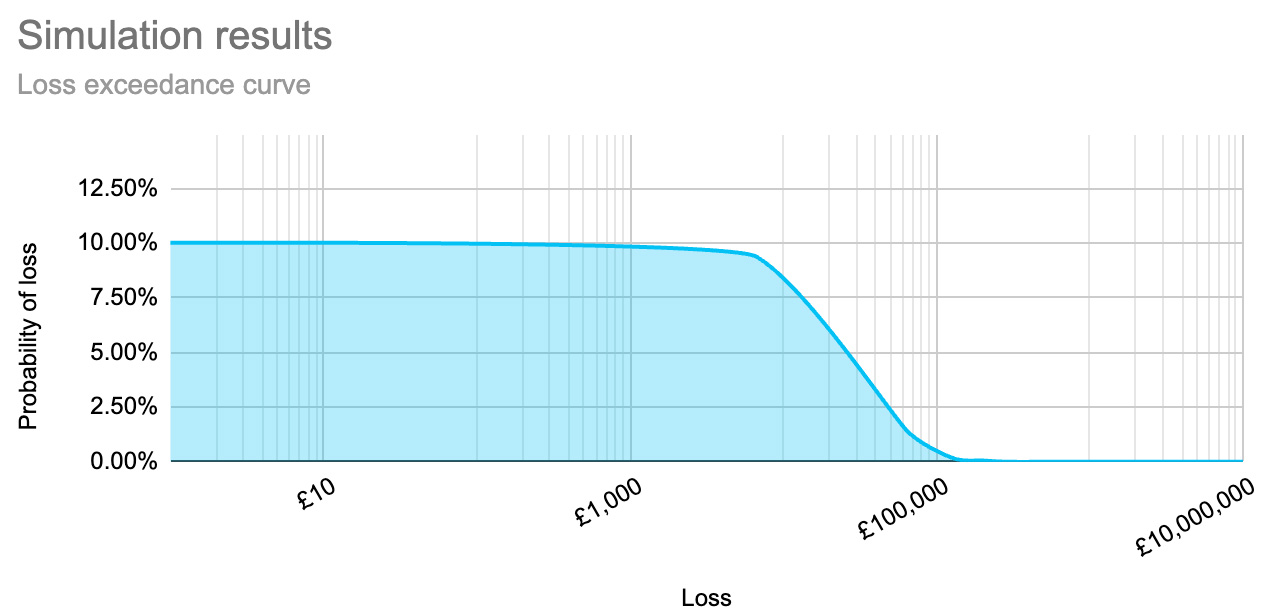
Fig. 7: Loss exceedance curve showing the risk from fig. 6.

Here we can see that while the overall likelihood hasn’t changed, the impact has decreased (the tail of the graph/slope has moved to the left).

How does this help?

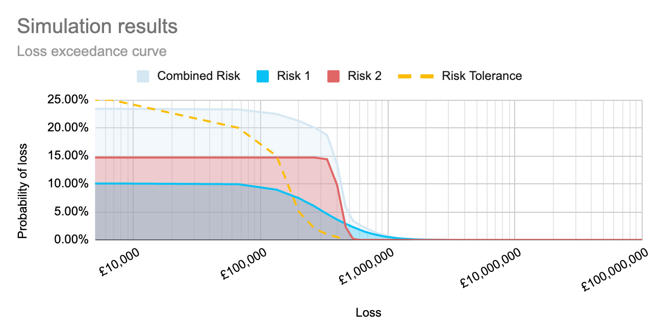
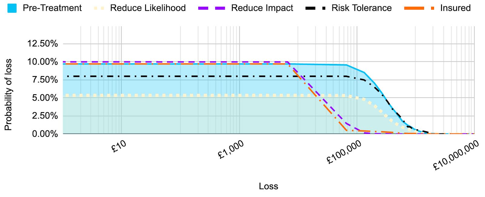
Well, let’s look at the effect of each control, compared to the inherent risk and the risk tolerance:

Fig. 8: Loss exceedance curve showing the comparison of the original risk, a reduced impact, and a reduced likelihood against the risk tolerance.

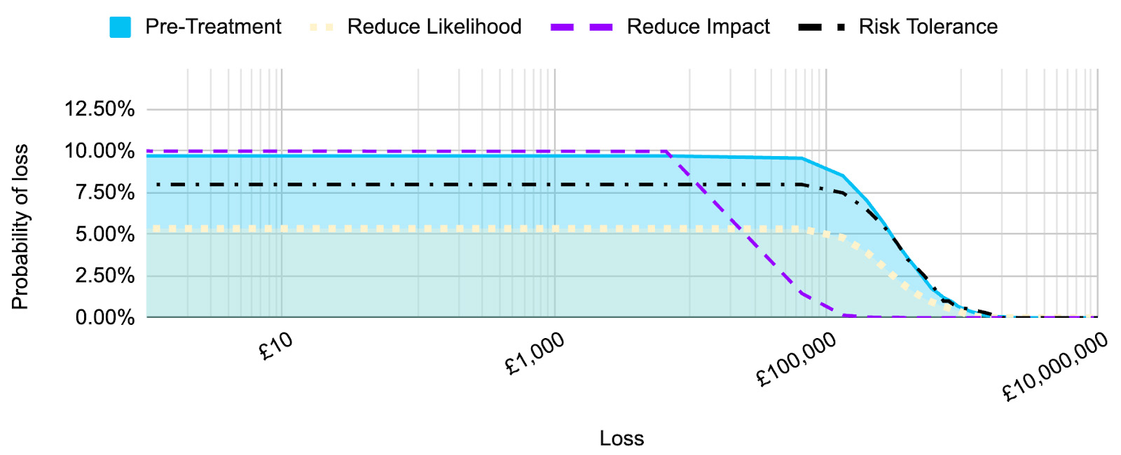
Here we can see that both the inherent (pre-treatment) risk and the residual risk after the control to reduce the impact has been implemented, are above the risk tolerance for lower level loss values. However, the control to reduce the likelihood of the risk being realised has reduced the risk to within the risk tolerance.

If I only had enough budget to implement one control, and this was the only risk scenario impacted by the controls, it would be much easier to justify why the control to reduce the likelihood of the risk being realised should be chosen over the control to reduce the impact.

Risk transfer

Contractual obligations and insurance are two of the most common ways that risks are transferred. In this post, we’ll consider how a cyber insurance policy can impact a risk profile.

For the simplification of the model, we make the following assumptions:

The policy excess and limit are applied equally to each event
There is no cost associated with making a claim on the insurance
The delay between the event and receiving payment from the insurer does not result in additional costs

Reduce impact within defined limits

When applying a risk transfer control, the initial risk calculation is unchanged. The events still occur as they would have without the risk transfer — it is afterwards that the impact cost is covered by the insurance company.

For this, the logic applied in the mathematical simulation needs the excess and maximum amount covered by the policy.

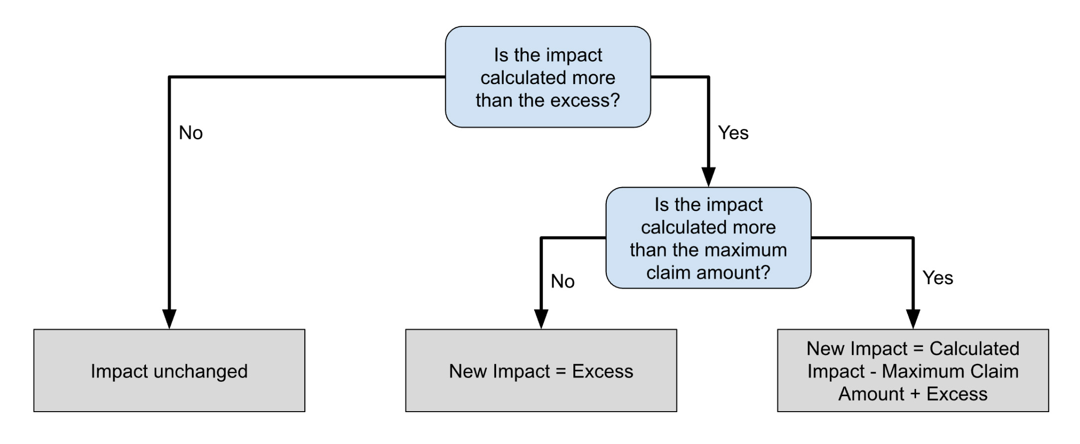
Fig. 9: Flow chart showing how transferring risk would affect the impact of the risk.

Once this workflow has been applied to all simulation results, we can see that the new risk profile shows a change in shape. In the profile below, we have applied an excess of £10k and a maximum claim value of £500k.

Fig. 10: Loss exceedance curve showing the application of the risk transference from fig. 9 on the risk from fig. 2.

In this amended profile, there is no change before the excess value is reached for any loss. Towards the tail end of the slope, we can see an area where the loss probability evens out (the line gets flatter) to show those risk events where the maximum claim amount has been exceeded and there has been a resultant cost for the organisation.

When comparing this to the other controls considered above, we can see that the insurance has a very similar impact on the risk profile to the control which reduced the impact of a risk event.

Fig. 11: Loss exceedance curve showing the comparison of the original risk, a reduced impact, a reduced likelihood, and a risk transference (insured) against the risk tolerance.

But that was just one insurance company, and we know they never offer the same terms, so let’s compare multiple insurance companies to see the impact of increasing the max claim and reducing the excess.

Here we have:

Insurance	Excess	Max Claim
Insurance 1	£10,000	£500,000
Higher Max Claim	£10,000	£100,000,000
Lower Excess	£5,000	£500,000

Table 1: Table of different insurance profiles.

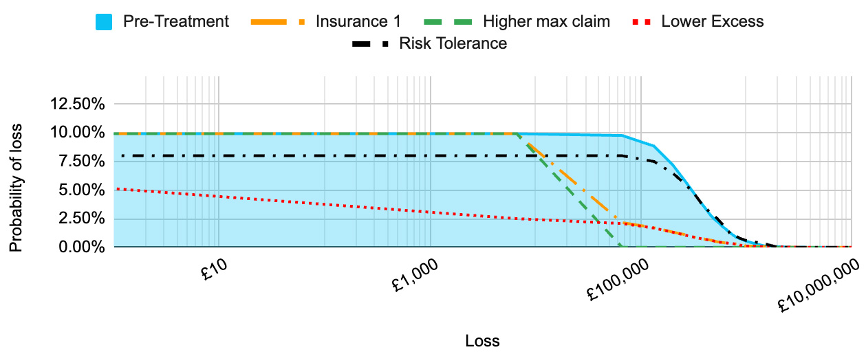
Fig. 12: Loss exceedance curve showing the comparison of types of insurance (from table 1) and how excess vs. max claim affects the risk profile.

Here we can see that increasing the max claim amount to 200 times the original insurance amount didn’t make much difference, and didn’t bring the risk profile to within the risk tolerance. However, halving the excess had a significant impact on the risk profile and brought it well within the risk tolerance.

Summary

Quantifying the effect that controls have on your risks can help you make the best choices for your organisation, when budgets and time don’t allow you to implement every control you would ideally want.

Up next

In a future post in this series, I will discuss how you can calculate the difference between the cost of a control and the expected reduction in costs associated with a risk.

Photo by Markus Winkler