The maths explained series: Quantitative risk analysis

In Qualitative and quantitative risk analysis, we talked about the difference between qualitative and quantitative risk analysis, and we made the case for the use of quantitative risk analysis in cybersecurity. In this post we will look to demystify the maths commonly used by other industries to calculate their risk, and show how the same methods can be used to provide a more meaningful view of your cybersecurity risk.

As mentioned in that earlier post, actuaries, portfolio managers, and other industries working with complex risk profiles use probability distributions, a form of quantitative risk analysis which provides a view of the probability of different impact values within a range of outcomes.

These distributions use the same information, from the same experts, that would be used in a standard risk matrix, but also utilise tried and tested statistical techniques to provide a more accurate view of the profile of each risk. That is, it is a model which acknowledges that there is a higher probability that a certain risk will result in a loss of £1,000 or more, than there is of the same risk resulting in a loss of £100,000 or more.

The model uses two main concepts:

1. A subject matter expert could, with a little guidance and training, provide a reasonable estimate for the financial impact of a cybersecurity event (this is at the very worse, no less accurate than the current system of them identifying which impact range an event fits into) - within a 90% confidence interval.
2. A cybersecurity event will never result in a negative loss, and so, as is commonly done for stock prices, can be modelled using a lognormal probability distribution.

Ok, what does any of that mean?

Let’s explain some terminology you may encounter when diving in.

What is a confidence interval?

A 90% confidence interval is just another way of saying that the expert is confident that 9 times out of 10 the impact of an event will fit between these 2 values. For more information on this, check out Jamie’s article on Why is estimating an important skill?

What is a probability distribution?

A probability distribution assigns a probability to each possible outcome, and for measurable outcomes (like cost) this is often shown as a graph. For business risks, it is usually a graph showing the likelihood of each monetary loss, for values in a set range, should a risk be realised.

To create probability distributions for cybersecurity risks, we utilise three main statistical concepts:

• Normal probability distributions
• Lognormal probability distributions
• Stochastic simulations (in particular Monte Carlo simulations)

Normal probability distributions

As the name suggests, these are the probability distributions which are normally seen, especially in nature. Human height, the birth weight of a puppy and the diameter of a tree are some of the many events whose values are normally distributed, and therefore the probability that a specific person, puppy or tree will be a specific height, weight or diameter can be modelled using a normal probability distribution.

These probability distributions are easily recognisable by the bell shape that they have when drawn as a graph. Imagine, for example, that we were to take all of the adult Springer Spaniels in the UK and weigh them. Adult Springer Spaniels usually weigh between 18 and 23 kilograms. If we were to plot all of their recorded weights, we would get a distribution that looks similar to the graph below. More dogs would weigh between 20 and 21 kilograms than between 21 and 22, or 19 and 20 kilograms. As you continue to move away from the centre of the graph, there would be fewer and fewer dogs who were measured to be that weight. So the probability of an adult Springer Spaniel being 18kg is lower than the probability of them being 20kg.

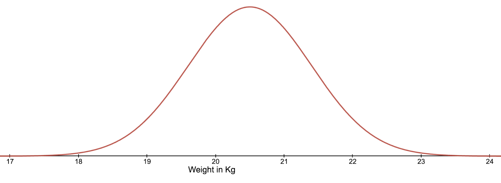
The symmetrical nature of this distribution type means that if we have just two values of equal probability, we are able to calculate both the mean (the most probable value), and the standard deviation (a standardised measure of how spread out the possible outcomes are). These two values are all that is needed to accurately replicate any normal distribution.

Lognormal probability distributions

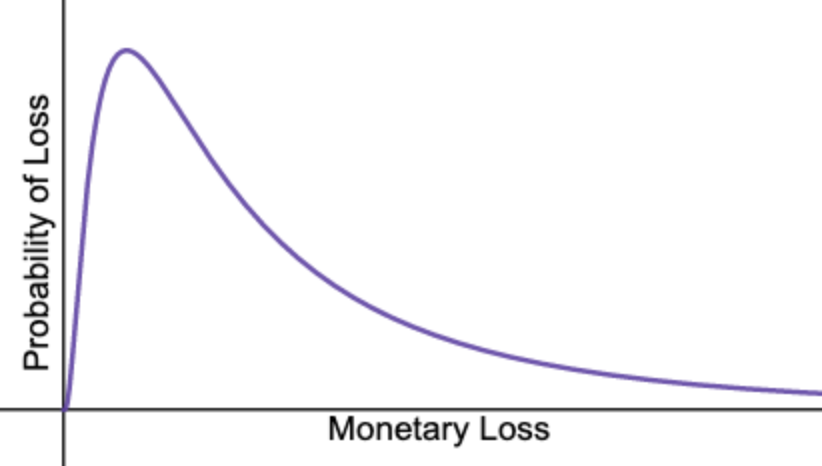
A lognormal probability distribution is not symmetrical, instead it has a long tail to the right which allows for the possibility of extreme events, and cannot have a negative value. Consider if we were to record the amount of prize money paid to gambling winners in the UK. The majority of prizes paid are relatively low (matching 2 or 3 numbers on the lottery or winning small amounts on scratch cards), however there are a very small number who win prizes of millions of pounds.

This model is also well suited for cybersecurity risk as the realisation of a cyber risk is never going to result in a negative loss, and there is always a small possibility of an extreme loss outcome.

A particularly useful feature of a lognormal distribution is that if you take the natural logarithm of the predicted values, and plot the distribution of these, you will get a normal distribution.

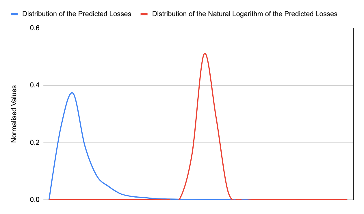
The relationship between a lognormal and normal distribution is bidirectional, which means we can use the characteristics of a normal distribution to calculate the location parameter (peak) and the scale parameter (spread of the distribution), by calculating the mean and standard deviation of the associated normal distribution.

So as with the normal distribution, only two values are needed to accurately reproduce the probability distribution. That 90% confidence interval, defined by the same SME who would decide which impact bucket a risk belongs in for qualitative risk analysis, is all the information needed to produce a probability distribution which will give a more nuanced view of risk.

Stochastic simulations

Stochastic simulations are simulated events, which incorporate randomness. This kind of modelling is used for many purposes including financial analysis, weather forecasting and biochemistry. One of the most well known stochastic models is the Monte Carlo simulation, a computerised simulation which utilises a random variable to simulate the probability of real-world events, while running the same scenario multiple times. Given the same initial conditions and parameters, different outcomes are produced on each run. It has been proven many times that this model, given a suitably high number of runs, is consistent with real world and expected outcomes.

How can these provide a view of cyber risk?

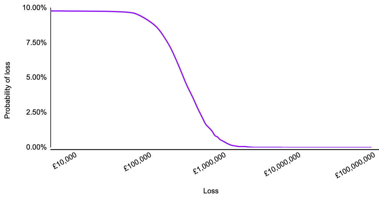
For cybersecurity risk modelling, we utilise a two-layered Monte Carlo simulation. First there is the probability that the event will occur at all, then there is the calculation of the event’s impact, based on the probability distribution described earlier. See the graph below for a risk that has a 10% chance of occurring.

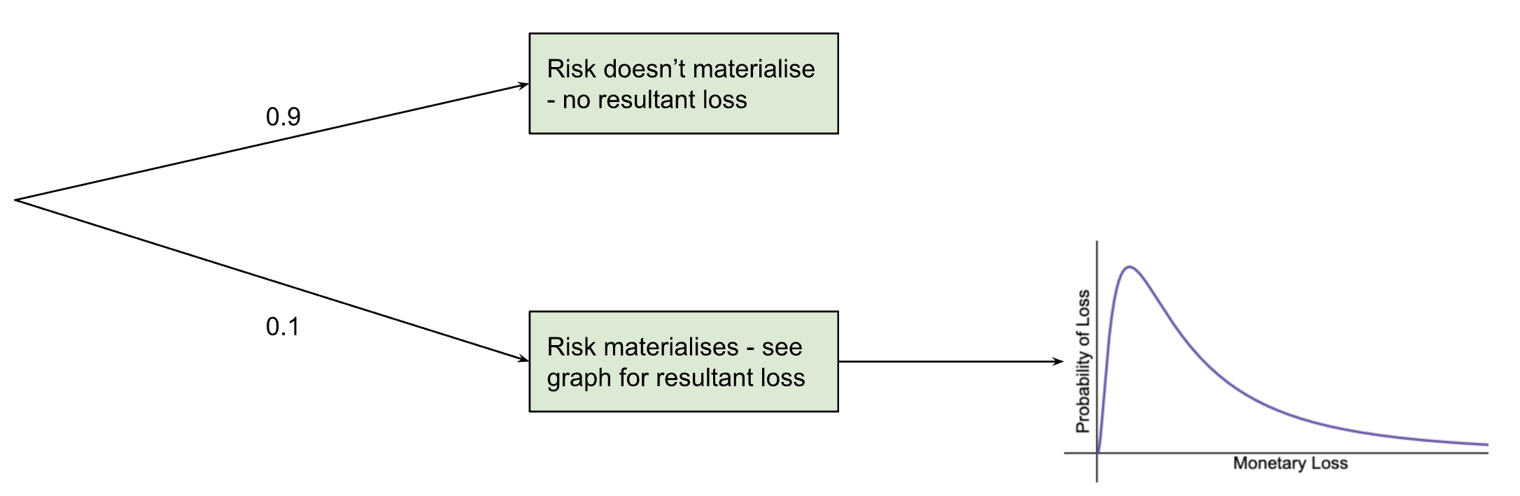
This means that the probabilities calculated for the graph only apply 10% of the time (so multiply them by 0.1) and the rest of the time the monetary loss (as a result of this specific risk) is zero.

It is relatively easy in Excel or Google sheets to then run a Monte Carlo simulation using these probabilities. The formulas used follow these steps:

• Pick a number between 0 and 1
• If this number is greater than the probability that the risk occurs (in this case, greater than 0.1), then the simulation marks that as the risk not occurring and records a loss of zero.
• If the probability is less than, or equal to the probability of the risk occurring, then we tell excel to calculate another random number between 0 and 1.
• Using that random number as the probability, and the location and scale parameters calculated earlier, excel returns the monetary value for that event occurring.
• This is repeated multiple times (thousands of times) and a graph of the results (counting how many are above each value) is produced to form a complete probability distribution for the risk.

This graph looks a little more like this:

The use cases and further usefulness of this method was described in the earlier blog post: Qualitative and quantitative risk analysis.

Questions?

Join Ray as he talks about this topic at his webinar on 7th September 2023, 12:30-1:30pm on Vimeo Live.

Photo by Scott Graham on Unsplash