Qualitative and quantitative risk analysis

Let’s start with some dictionary definitions:

Qualitative, adj: “based on information that cannot be easily measured, such as people’s opinions and feelings, rather than on information that can be shown in numbers”

Quantitative, adj: “related to information that can be shown in numbers and amounts”
- Cambridge Business English Dictionary

So, qualitative refers to things you can’t specifically count. Quantitative refers to things you can.

Qualitative vs. quantitative - what’s the real difference?

Young children, when given coins, start by counting their coins and being happy that they have x number of coins. A slightly older child might recognise that silver coins are better than brown coins. Their older sibling however knows the value of each coin and can increase the amount of money they have, without upsetting their siblings, by swapping multiple lower value coins for others of higher value.

Children start with a qualitative understanding of money before moving to a more useful quantitative understanding.

In cybersecurity, we tend to relegate our risk analysis to the realm of very qualitative analysis: using RAG ratings, educated best estimates, and resorting to wide impact ranges to try and cover every possible outcome.

Information that, at its core, is numerical in nature (probabilities, financial impacts, etc.) is wedged into colourful boxes that reduce measurable data into boxes that can only be counted.

Like children learning to use money, there’s a similar struggle with risks that have been relegated to boxes with descriptions like “Low”, “Med”, “High”. For example: how many low risks does it take to be worse than a medium or high risk? Within those categories, how do you know which risk is having the greatest impact on the business?

Better to be shotgun accurate than stormtrooper precise

Lots of people believe that the risks associated with cybersecurity are too complex to calculate precisely, so quantitative risk analysis would be too inaccurate to add value. The truth is that it’s possible to do basic quantitative risk analysis using the same expert knowledge that you would use for basic qualitative risk analysis. The result is a slightly more accurate measure of an organisation’s risk.

The methodologies are well known, and have been tested and refined by other industries. Actuaries, portfolio managers, and other industries working with complex risk profiles use probability distributions, a form of quantitative risk analysis which provides a view of the probability of different impact values within a range of outcomes.

These distributions use the same information, from the same experts, that would be used in a standard risk matrix, but also use tried and tested statistical techniques to provide a more accurate view of the profile of each risk.

What you end up with is a model that, for example, acknowledges that there’s a higher probability that a certain risk will result in a loss of £1,000 or more, than of the same risk resulting in a loss of £100,000 or more.

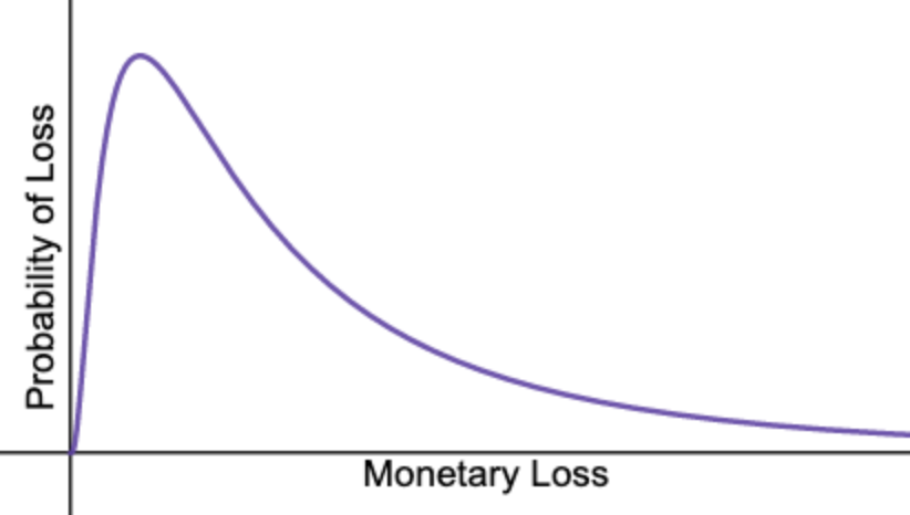
Probability distribution graph

What does that look like in practice?

For cybersecurity risk modelling, we utilise something that statisticians call a “two-layered Monte Carlo simulation”. First there is the probability that the event will occur at all, then there is the calculation of the event’s impact, based on the probability distribution described earlier. See the graph below for a risk that has a 10% chance of occurring.

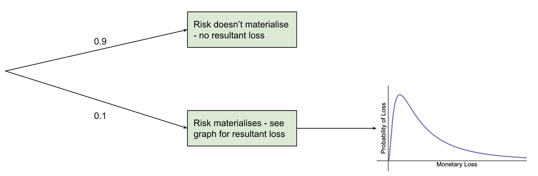
This means that the probabilities calculated for the graph only apply 10% of the time (so multiply them by 0.1) and the rest of the time the monetary loss (as a result of this specific risk) is zero.

In simple terms: there’s a small risk, some of the time. But most of the time, there’s no risk at all.

You can go further. It’s relatively easy to run a simulation in a spreadsheet using these probabilities. This involves running the same scenario, with the same probabilities, over and over again to approximate the real world results. This produces an annualised probability distribution, which looks a little more like this:

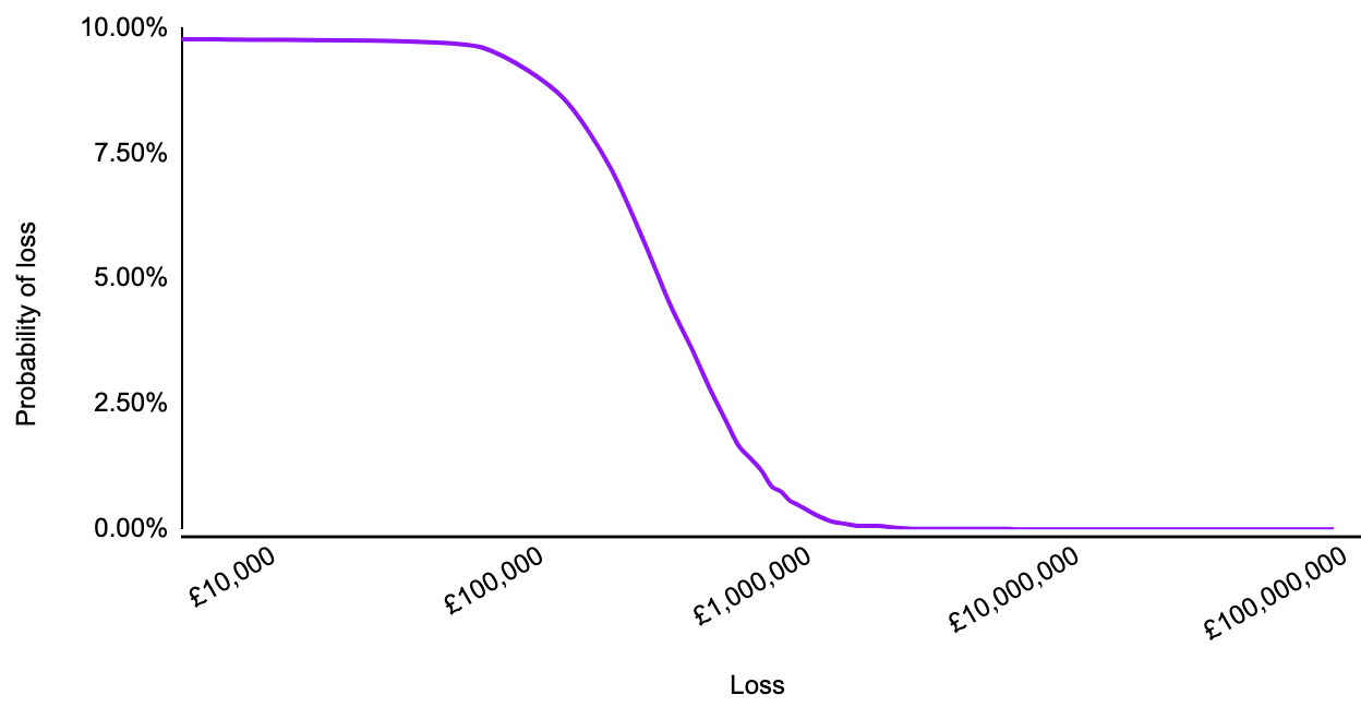
Why is that useful?

At surface-level this might not appear to be any more useful than the qualitative risk analysis - at least everyone knows what the red, amber and green mean, right?

The value of this methodology, and the graphs you create with it, is in what you can do next.

Do you have a set of controls that you’re considering implementing? Then run the same methodology, defining an event likelihood and 90% confidence interval for impact based on the assumption that the controls are implemented.

We can now graph these two probability distributions together. This provides a good visual representation of where an unmitigated risk profile exceeds the organisation’s risk tolerance (where the pre-treatment graph is above the risk tolerance line). It also shows whether proposed controls/mitigations are likely to bring the risk to within tolerance levels.

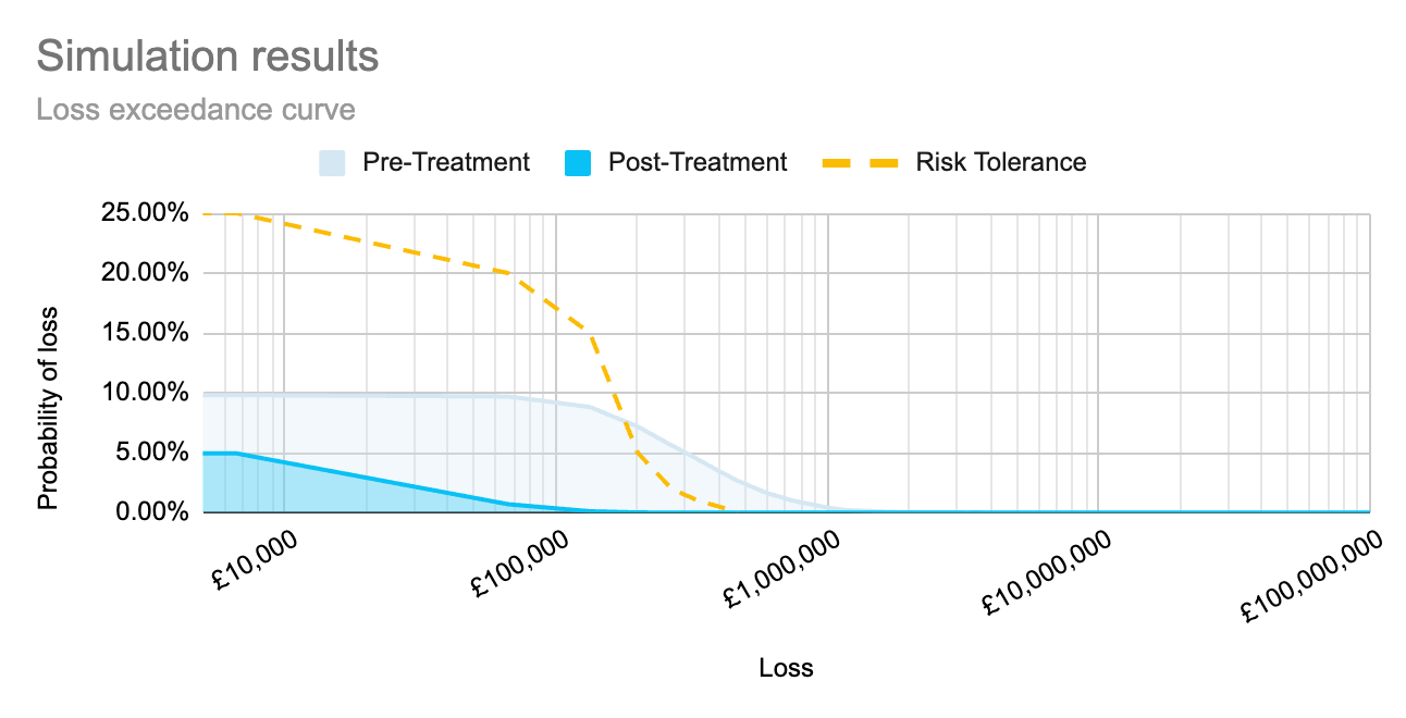
For a quick and easy way to see what this could look like for your organisation, register for access to Cydea’s risk app.

Further usefulness

Do you have multiple risks and a limited budget? Do you need to know which controls are likely to provide the biggest impact to your overall risk profile? Do you want to be able to quantify/demonstrate the impact that implemented controls are having?

As we are using numbers and statistical simulations it is possible to combine the probabilities of multiple events, including situations where the realisation of one risk increases the probability of another, or combining multiple independent events which can be mitigated by the same control.

The upshot is more meaningful views of risk rather than a discrete count of high, medium or low risks.

These views, whether for individual or combined risks, can then be used to:

• help with the prioritisation of cybersecurity budget to those areas where they’ll have most impact
• justify cybersecurity spending
• identify areas of high risk

Photo by Glenn Carstens-Peters on Unsplash