What do you do when there’s more than one risk?

What do you do when there’s more than one risk?

Let’s do a little thought experiment. Imagine that you’re in charge of controlling cyber security risks in your organisation, and that you can only afford to implement one control this quarter. Which one should you implement: the one that will mitigate a high and 2 mediums down to 3 lows, or the one that will reduce 3 highs down to a medium and 2 lows?

In my post about Qualitative and quantitative risk analysis, I discussed how quantitative methods could be used to assign a numerical value to risks. I also looked at how these methods could be repeated to allow for comparison, for example, comparing inherent and residual risks.

As we all know though, individual risks rarely sit in isolation, and the controls implemented to remediate one risk will likely have an impact on multiple risks. So how do we calculate the compound risk? For this post, we will only consider the impact to likelihood of combining risks and assume that the realisation of one risk does not change the impact of another.

Why can’t we just add them together?

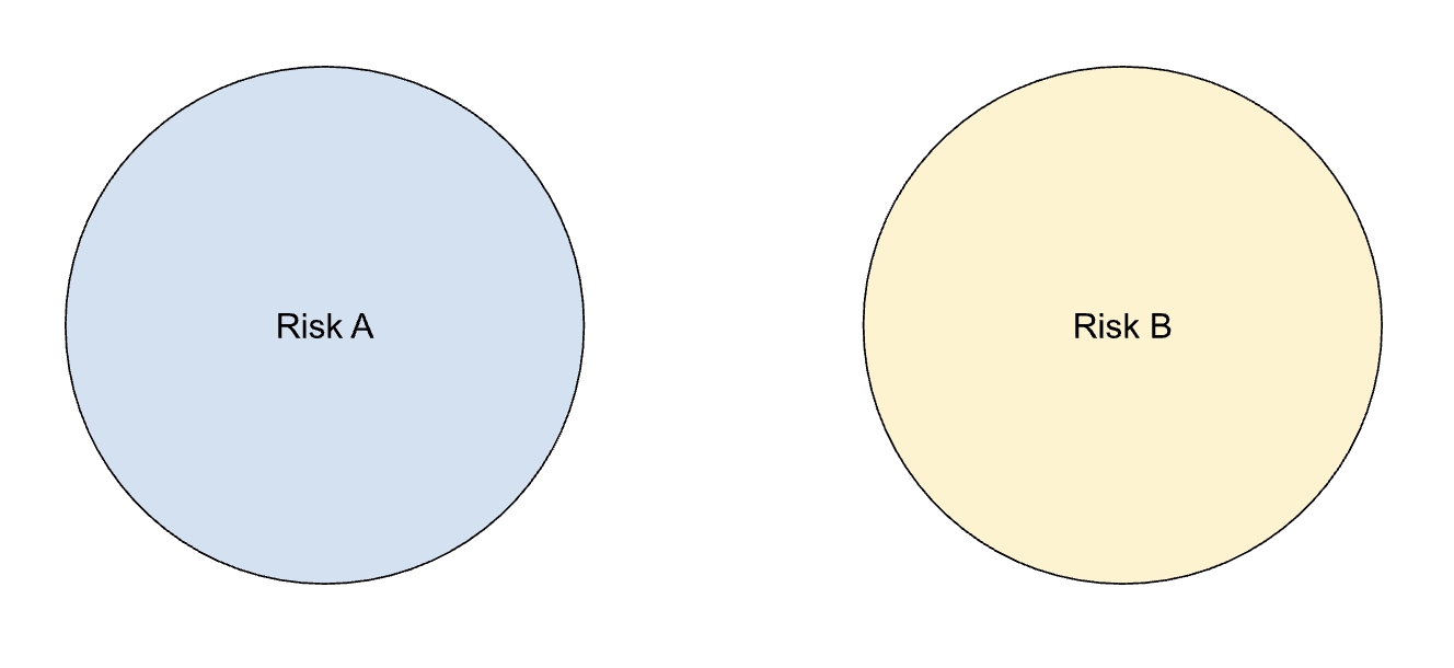
You can, but only if the risks are mutually exclusive. That is, if one risk being realised precludes the realisation of the other. Let’s take a look at two risks: Risk A and Risk B.

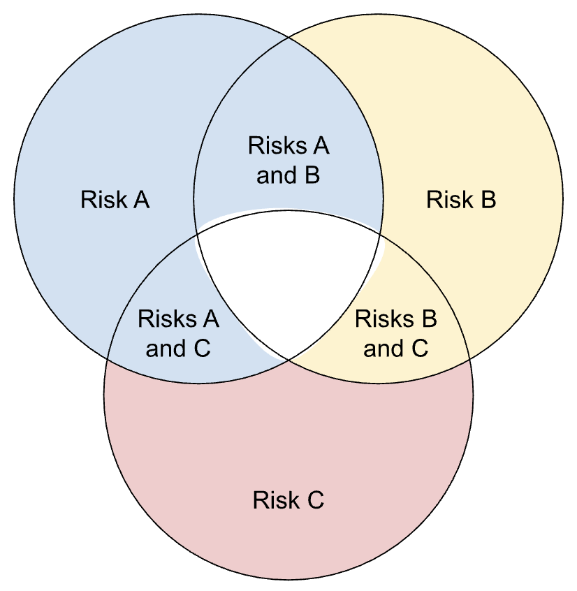
Let’s look at why we can’t just add the risks together if they are not mutually exclusive, so if there is always the possibility that both risk A and risk B will occur. This is shown by the overlapping circles:

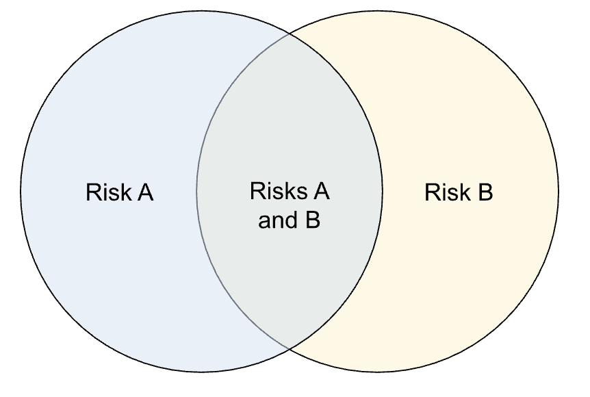
We can see in the image above that if we just add the areas of the two circles together to get the area of the combined shape, we end up counting the area that overlaps twice. This is the same thing that happens if we just add the probabilities of the two risks occurring together: we end up counting the probability of both risks occurring twice.

So when calculating the combined risk, we add the probabilities together and subtract the probability of both events occurring to remove the double count. This is known as Bayes theorem.

This theory can be expanded to 3 or more risks:

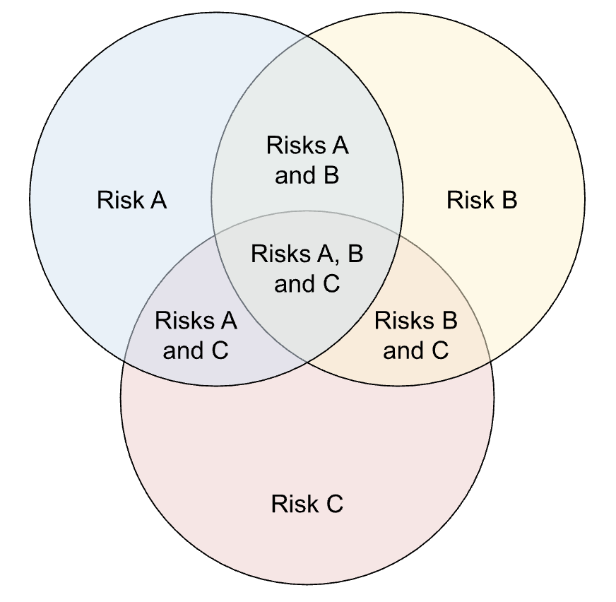
The same initial process is followed, adding all of the risk probabilities together and subtracting the probabilities for each pair of risks (risk A and B; risk B and C; risk A and C). The difference with 3 or more risks, is that there are the same number of risk pairs as there are risks.

So the probability of all of the events happening ends up being deleted when the pairs of risk events are subtracted, as illustrated below, and this must be added back in to avoid this missed combination of events.

No matter the number of risks included in the calculation after 3, this process remains the same.

Why is this useful to know?

Ok, so we know the total likelihood associated with a group of risks. What can we do with that?

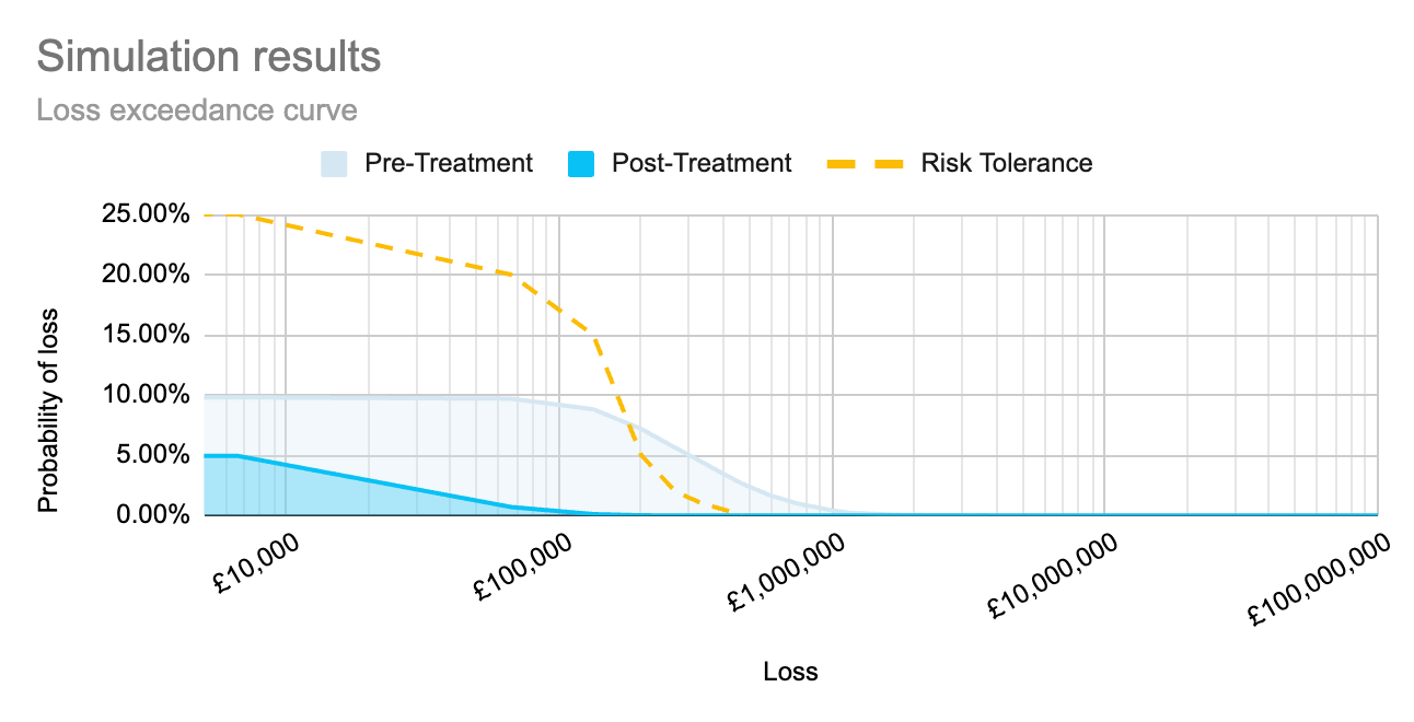
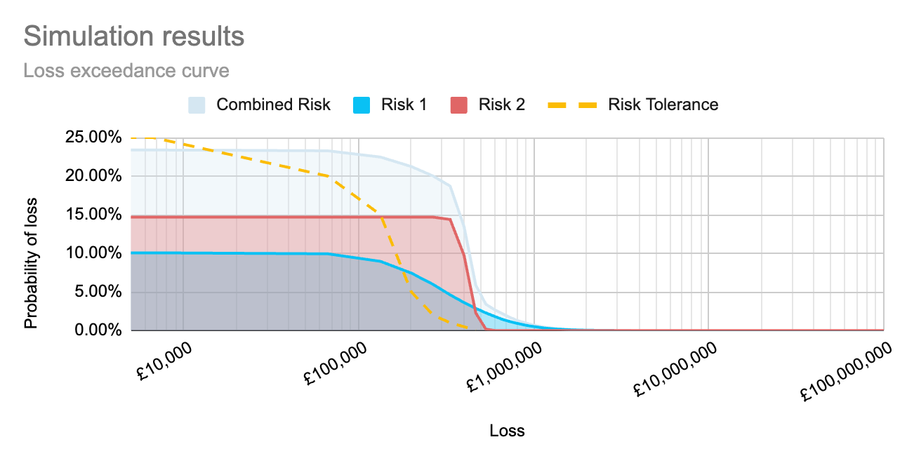
As I wrote in Qualitative and quantitative risk analysis, running simulations to calculate each risk separately, as well as simulations to calculate the compound risk, creates the graph below. It shows how both individual risks and combined risks sit within the organisation’s tolerance. That means we can see the full impact of implementing a proposed control, both on individual risk scenarios, and as an aggregate across multiple impacted risk scenarios.

For a quick and easy way to see what this could look like for your organisation, register for access to Cydea’s risk app.

As you can imagine though, if you opt to make these simulations within a spreadsheet, the formulas can quickly become complex, and it is easy to mistype something. So, as with creating any mathematical model or simulation, it is important to have an idea of what outcomes could be reasonably expected to be produced by the model.

That’s where this understanding of the expected total probability comes into play. If we look at the graph above, we can see that the probability of loss associated with the combined risk is slightly less than the sum of the probabilities of the individual risks, as expected.

If you want to know more about the maths behind this topic, keep an eye out for the next post in our Maths Explained series.

Headline photo by Belinda Fewings on Unsplash